Classifying all of the pdfs on the internet

TLDR:

I classified the entirety of SafeDocs using a mixture of LLMs, Embeddings Models, XGBoost and just for fun some LinearRegressors. In the process I too created some really pretty graphs!

Introduction

How would you classify all the pdfs in the internet? Well, that is what I tried doing this time.

Lets begin with the mother of all datasets: Common Crawl or CC is a web archive of all of the internet, it currently is petabytes in size and has been running since 2007. Maybe, you know about the Internet Archive which is almost the same but with the main difference being that Common Crawl focuses more on archiving the internet for scientists and researchers instead of digital preservation.

What this translates into is that CC doesn’t save all of the pdfs when it finds them. Specifically, when Common Crawl gets to a pdf, it just stores the first megabyte of information and truncates the rest.

This is where SafeDocs or CC-MAIN-2021-31-PDF-UNTRUNCATED enters the picture. This corpus was originally created by the DARPA SafeDocs program and what it did was refetch all the different pdfs from a snapshot of Common Crawl to have untruncated versions of them. This dataset is incredibly big, it has roughly 8.4~ million pdfs that uncompressed total 8TB. This corpus is the biggest pure pdf dataset on the internet¹.

So I tried classifying it because it doesn’t sound that hard.

Dataset generation

Lets define what classifying all of this pdfs using different labels actually means. For example: I wanted to tag a Linear Algebra pdf as Math or an Anatomy textbook as Medicine.

The reason for all of this is because I wanted to use LLMs in my personal projects and I got this idea after reading the Fineweb technical blog / paper. The FineWeb team endedup creating a subset for “educational” content based on the bigger FineWeb dataset. What they did was use a Teacher and student approach where the LLM generates labels from unstructured text and then you train a smaller student or “distilled” learner capable of classifying based on the labels generated.

So I decided to follow the same approach. The problem is that 8TB of data is still a lot of information. I don’t have 8TB laying around, but we can be a bit more clever. The original dataset has the metadata available for download. Its only 8GB of pure text!

In particular I cared about a specific column called url. I really care about the urls because they essentially tell us a lot more from a website than what meats the eye. For example:

https://assets.openstax.org/oscms-prodcms/media/documents/Introduction_to_Python_Programming_-_WEB.pdf

Specifically this part:

Introduction_to_Python_Programming_-_WEB.pdf

Tells us a lot of information.

I know that this url is going to be education or technology adjacent. For now, lets just say its education because it has the “Introduction” part in its name.

Here is where the bit of prompt engineering that I used enters the picture.

Few shot prompting

Few shot prompting is a fancy name for making an LLM learn with examples without training it. Its a really cool trick that you can use to make the models outputs more coherent and consistent. I am going to give you an extremely easy example of how one of this prompts look like:

This might feel like magic if it is the first time you are using it, but LLMs are incredible at following patterns and just showing how to do things can make it improve their performance.

Using this method I generated 100k labels (to start) using this specific prompt and the Llama-3-70B model through the together API.

The distribution of 100k labels looks originally like this:

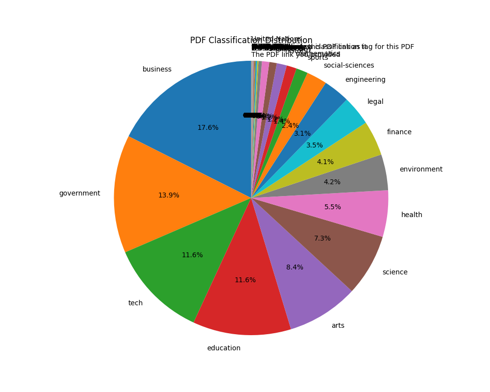
So, as you can see, there is a lot of really small data points that are going to be extremely annoying to classify. So guess what I’m going to do? I’m going to ditch anything with less than 250 labels and label them as other just to keep the most frequent classes.

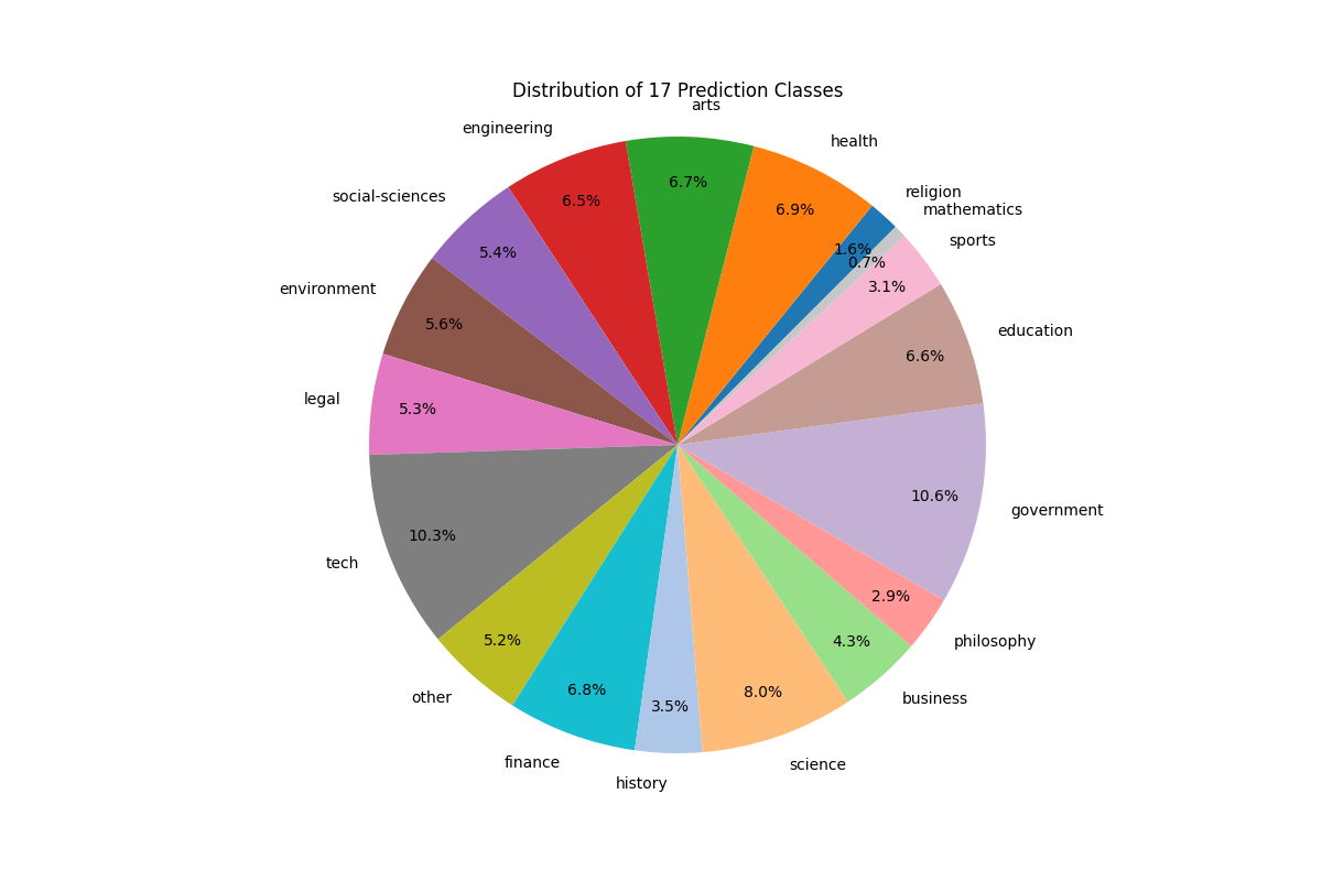
Because this labels are unbalanced, I decided to balance them and just take 5k samples at the most of each possible label. This left me with a total of 59k labels:

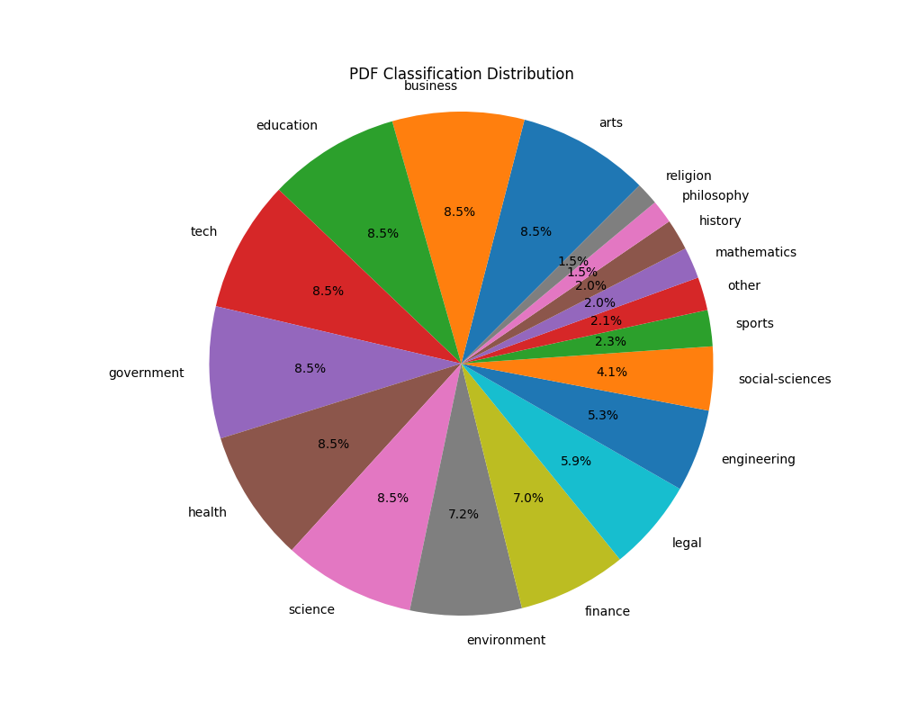
With this newly minted dataset, I decided to start going after the training of the new student classifier!

Model Training

Idea 1

I am going to introduce the idea of an embeddings model. For short, an embeddings model is a model capable of passing things like text, images, video or any other “unstructured” information to vectors in an ndimensional space with semantic meaning. In other words, you can have some points that are near each other like dog, cat, elephant and this ones are going to be separated from something like car, truck or vehicle.

With that in mind, this models are great for generating clusters of meaning. This is going to be extremely useful for us, because we are going to just make this model be capable of classifying the specific labels that we ended up having through a process called finetuning.

Finetuning is were you grab an already trained model for a generic task and just train it a little bit more for your particular problem. This case being classification. If you want to learn more about finetuning you should check out the first fast.ai lecture where they finetune a model.

In the FineWeb paper, they used a total of 500k labels. Thats a lot more than what I currently had, but at the time, I decided to ignore this². I went on with my life and decided to just start testing some models. And oh boy, I realized that you can do a lot with just a gaming laptop.

In FineWeb Edu they used a specific embeddings model based on the snowflake-arctic-embed-m. But it is not the best embeddings model based on the Massive Text Embeddings Benchmark. So I decided to try some models that ranked really well in here. The problem with this benchmark is that most of the models are too big, with roughly 7B parameters, I can not afford to run that and expect it to classify 8 million pdfs quickly. So I decided to instead go for the next best thing, Stella_en_400M. But the problem was that I wanted to read how it worked and I don’t really like when a model is published and you go to a Github link that has a TODO: add the rest of info in their README.

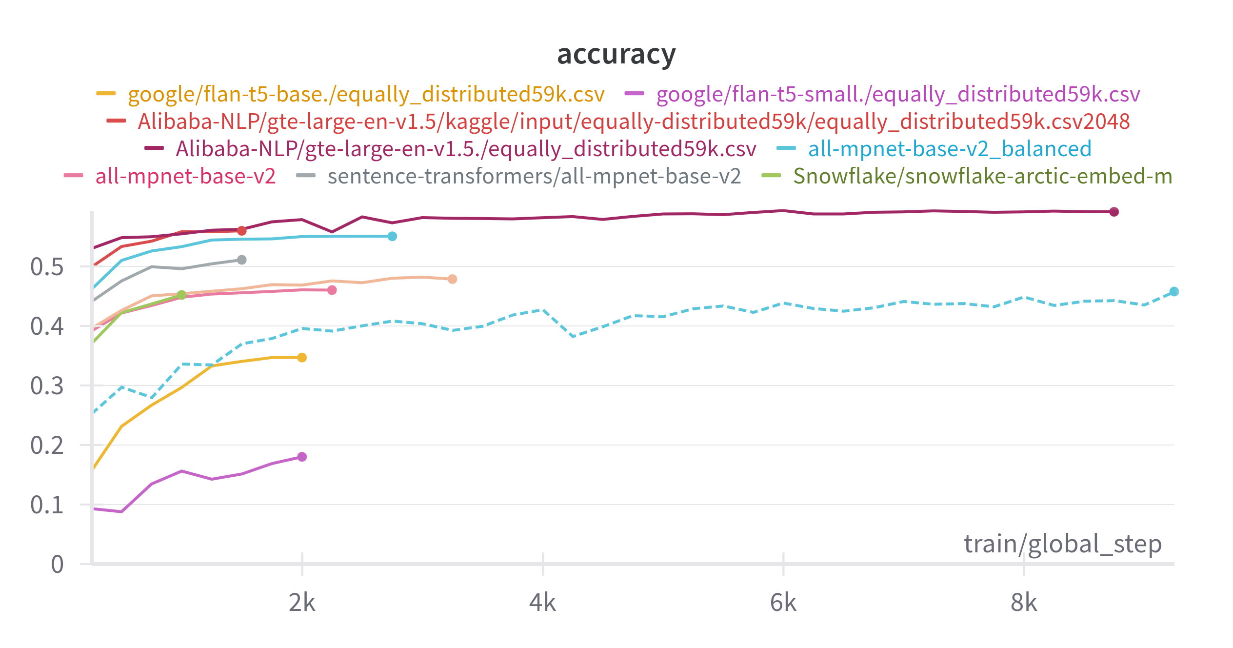
So, I decided to try out a range of models including the base model for Stella called gte-large-1.5 and Arctic Embed. Along with others like all-mpnet-base, distillbert, flant-t5-small and bert-base-uncased.

Finetuning a model is pretty simple with Huggingface because it abstracts a lot of the code from you and thanks to just freezing the main model and training the embeddings and the classifier head I could run the entire thing in my laptop without the need of an external GPU³. After a series of runs, I found that for my problem the most performant model was Alibaba-large-gte-1.5, it got up to 59.14% of accuracy.

I was a bit disappointed at this point because I had paid for a bunch of labels and it seemed that I needed to be more careful on the training or generate a bigger dataset.

But in my true lowest moment, I remembered that XGBoost existed. Yes, this story is going to become an traditional ML story.

Idea 2

For those of you in the know, you could see this coming, XGBoost is THE undisputed king of tabular data, it currently is the state of the art. If you don’t know the internals for XGBoost, I’m not explaining it in detail but don’t worry about it, the StatsQuest Youtube Channel has an amazing series of videos where they explain them in like two hours.

For now, think about XGBoost as the if else version of AI. They are THE simple transparent box that classifies extremely well.

This time, I am going to reframe the problem. Do you remember that the model that I used in the first place was really good at generating this embeddings? Well, what if this embeddings could be used to train another model? What if we could pass from having text to training on tabular data? This time the pipeline to train the model would look like the following:

Another big extra from this would be that I can run a lot more experiments because training an XGBoost model is way faster than training an embeddings model. So I decided to generate all of the embeddings for the PDF links. Generating all of the embeddings is a total of 40GBs uncompressed.

Finally, the last change that I decided to do was to train simpler models. Instead of training a big classifier, it could potentially be better to just train a binary classifier per class. This idea I learned from an old Kaggle competition. Thanks you Chris! The main idea behind this is to have tiny models that are really good capable of super fast inference for specific problems, instead of trying to solve all of it with just one big model.

With this in mind, the combined models have this as result!

Average Performance:
accuracy     0.839750
precision    0.859758
recall       0.819733
f1           0.838937

This approach is already winning against the original naïve deep learning approach that I had by 24.83%.

Idea 3

But guess what? You don’t actually need deep learning to generate embeddings. You can just split the text into smaller parts and count the occurrences of it. There is a this thing called TFIDF (Term Frequency-Inverse Document Frequency) that is almost that but it has a fancier formula. TFIDF is a numerical statistic that reflects how important a word is to a document in a collection. It’s calculated as:

TFIDF(t,d,D) = TF(t,d) * IDF(t,D)

Where:
TF(t,d) = (Number of times term t appears in document d) / (Total number of terms in document d)
IDF(t,D) = log(Total number of documents in corpus D / Number of documents containing term t)

This method assigns higher weights to terms that are frequent in a specific document but rare across the entire corpus, making it great for feature extraction in text analysis. So I decided to go full on out and just go back to the basics of NLP. To my surprise, the resulting models where not complete garbage!

They were actually capable of predicting something that wasn’t as bad as I was expecting:

Average Performance:
accuracy     0.675200
precision    0.683185
recall       0.646316
f1           0.662497

Better than my naïve approach!

I even trained a Linear Regressor ensemble that is better than the baseline deep learning model.

Average Performance:
accuracy     0.706802
precision    0.723558
recall       0.663038
f1           0.690286

This is the moment where I felt that I messed up and I should have gone back to the basics. If the point of this was actual production, I would be happy with this models!

But lets be real, I am just having fun in here, I don’t really care about what is the best, I want to try new things and I won’t let Deep Learning down.

Idea 4

Back to the world of Deep Learning, at the end of the day, all of this are just experiments and I wanted to see how far I could stretch my capacity of using a single Deep Learning Classifier. My goal was extremely simple. I wanted to get to at least 70% accuracy.

The first thing that I made was generate a lot more labels, I feel like I did Deep Learning a disservice by using so little data. So I generate another 400k labels using Llama3.1-7B (this time a smaller model because I don’t want to break the bank on inference).

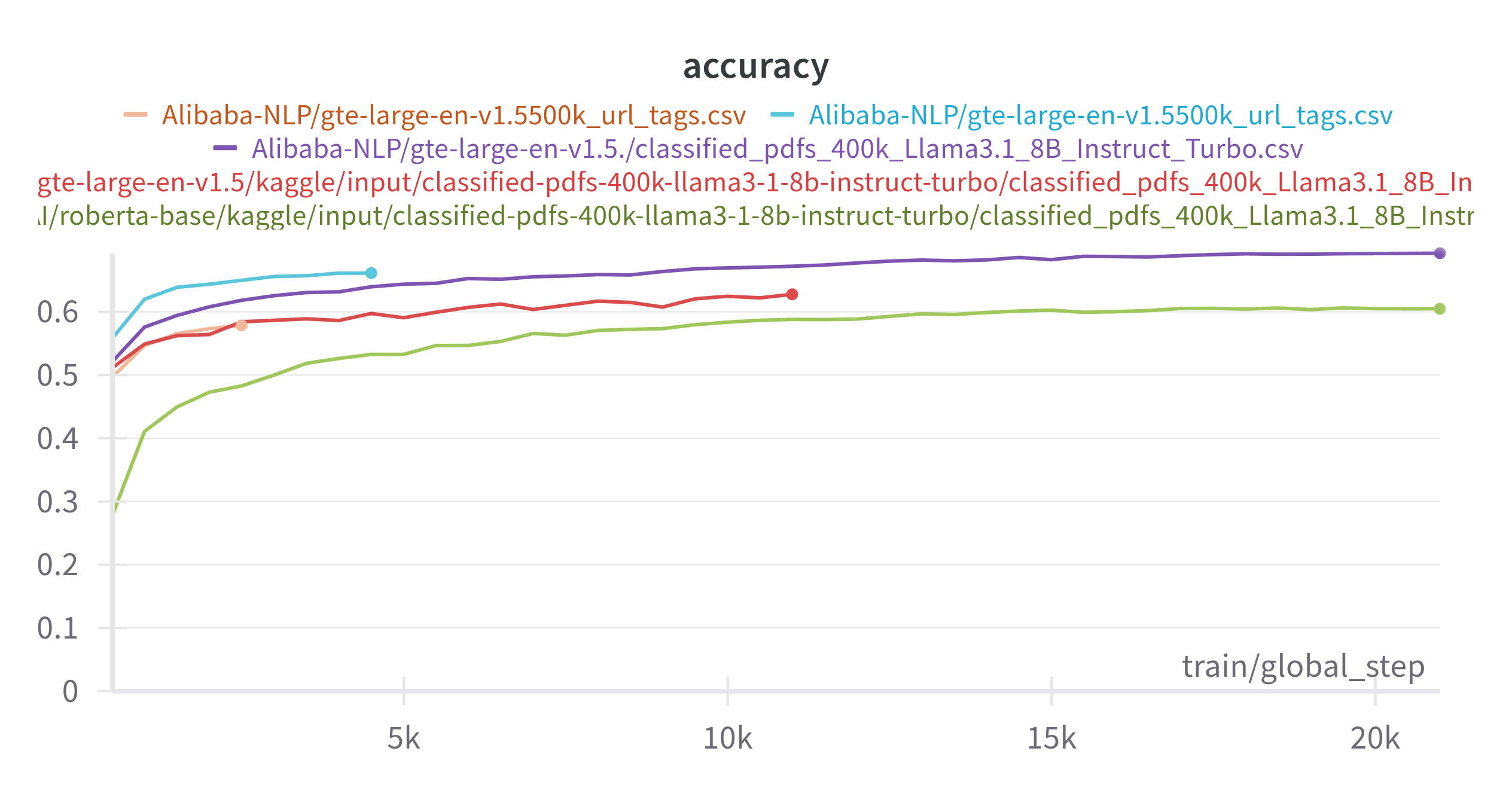
I did some experiments and to not bore you I saw that the more data the better for my specific runs. So I decided to just do a dry run with two different models, this time, influenced by the The Llama 3 Herd of Models from Meta I used the roberta-base model and the good old gte-large from before.

gte-large got me a lot closer to what I was expecting with results of up to 69.22% accuracy on the training dataset[2].

Results from experimenting

Here are the performances of all of our models!

Model Name	Accuracy
gte-large naïve (59k labels)	59.14%
xgboost embeddings	83.97%
xgboost Tf-Idf	67.52%
LinearRegressor Tf-Idf	70.68%
gte-large naïve (400k labels)	69.22%

I genuinely think that it was a skill issue from my side that I was uncapable of making the Deep Learning model perform at the top of the performance chart. Anyways, for now I am just going to grab the best model which was the XGBoost embeddings model and really dial it in because I want to do other projects in my free time.

Hyper Parameter Sweep

The last thing that I tried was a hyper parameter sweep on the XGBoost embeddings model because it was the most performant overall. A hyperparameter sweep is basically a way to move all the different nobs that the base model has so that it can perform to the best of its abilities.

Model Name	Accuracy
gte-large naïve (59k labels)	59.14%
XGBoost embeddings	83.97%
XGBoost Tf-Idf	67.52%
LinearRegressor Tf-Idf	70.68%
gte-large naïve (400k labels)	69.22%
XGBoost Embeddings HyperParameter Sweep	85.26%

Now that we have some models, we can do the fun part and generate labels for the rest of the entire dataset!

Classifying all the corpus

The code is nothing fancy. It literally loads to memory some embeddings and then predicts them. The distribution of predictions looks like the following:

It took roughly an hour to predict all of the pdf tags but this was because I didn’t make it run on GPU because I forgot to set it up that way. But even then, I would have to say that it is not that bad times wise!

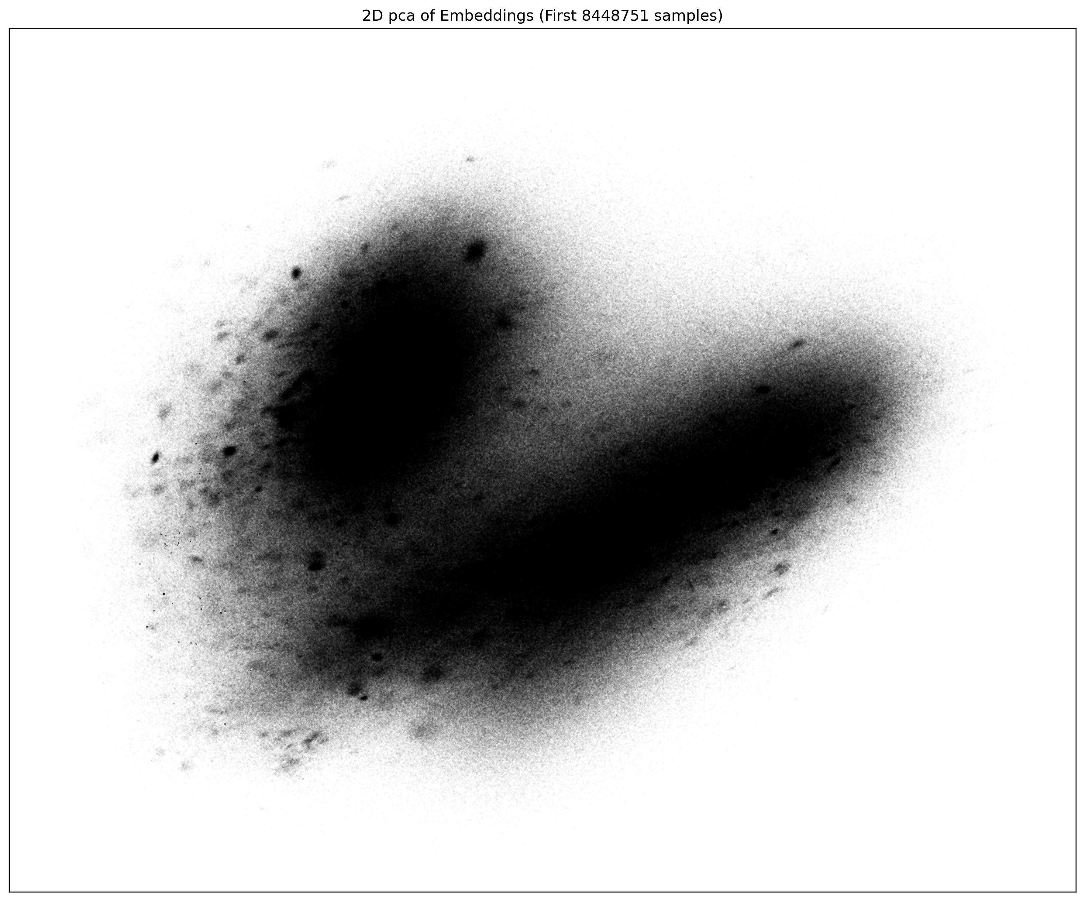
Finally, I wanted to generate some incredibly aesthetically pleasing pictures. And after doing some test runs on my local machine I decided to do some PCA and UMAP visualizations of a looot of points. Like, ALL of the predictions + embeddings. I am pretty sure this are not the biggest runs of PCA and UMAP but they might be up there.

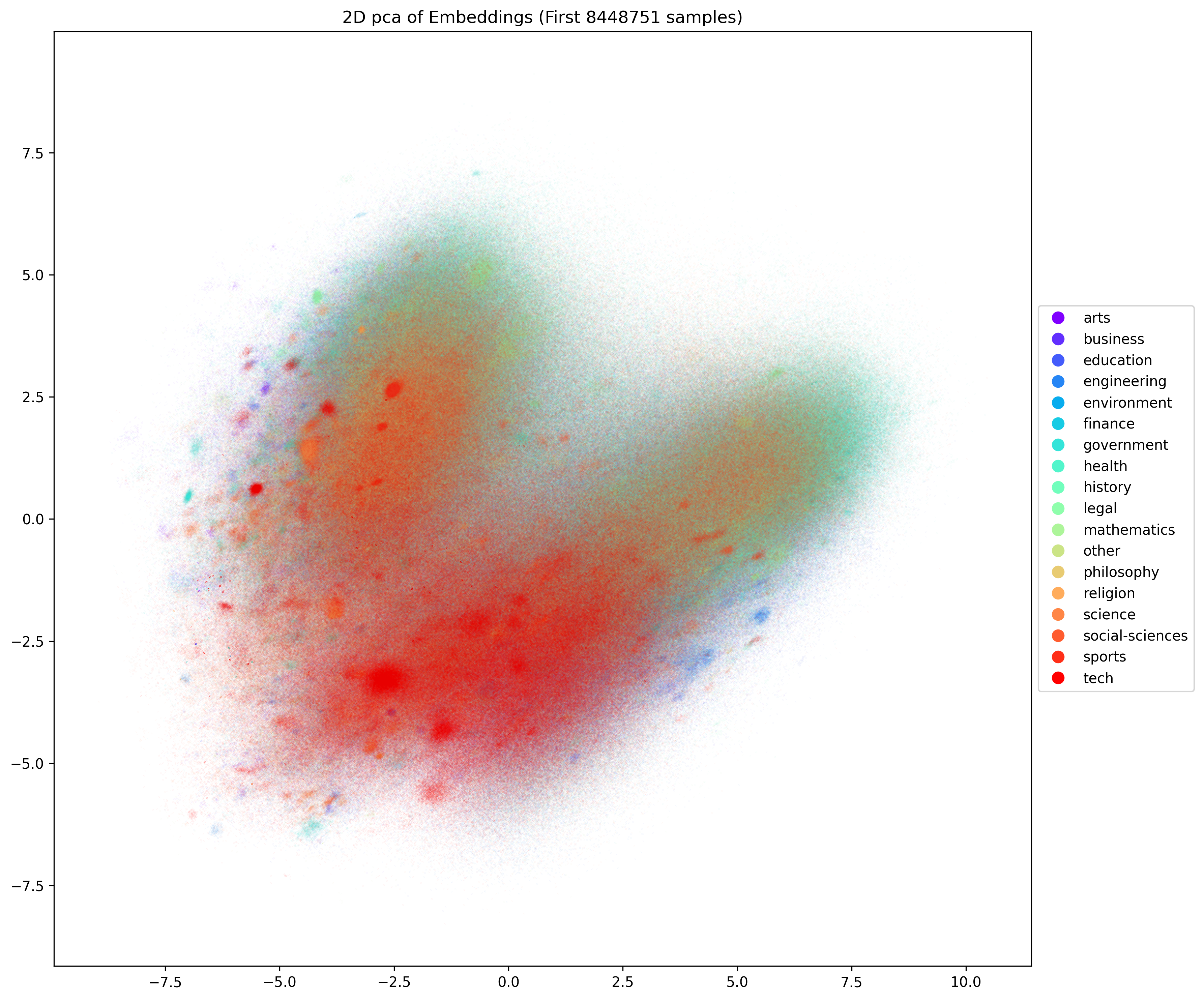
For PCA I made a visualization of the entire dataset. All of the eight and a half million dots in a single picture:

For the classifications, it looks like this:

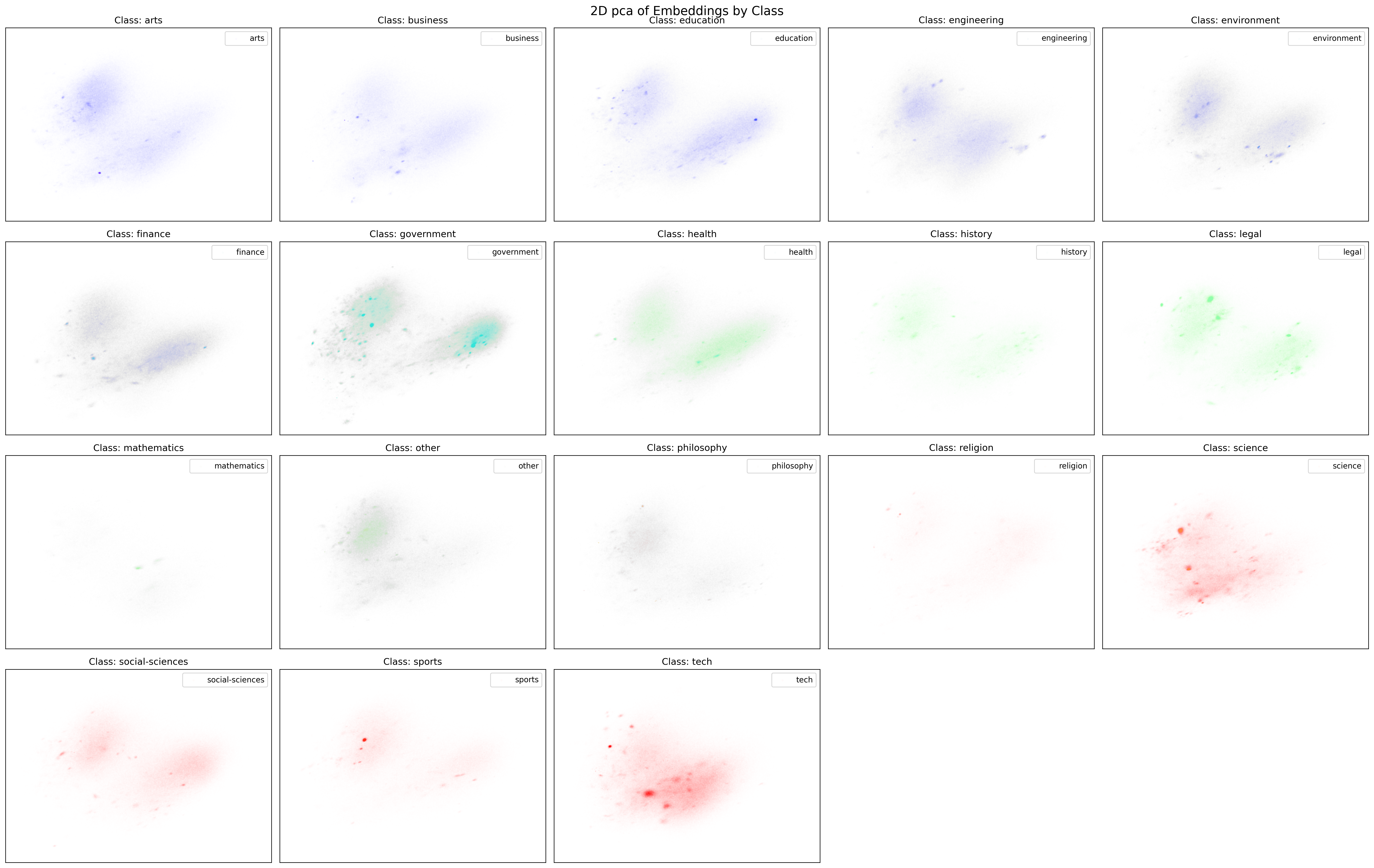
And if we decouple each class it looks like this:

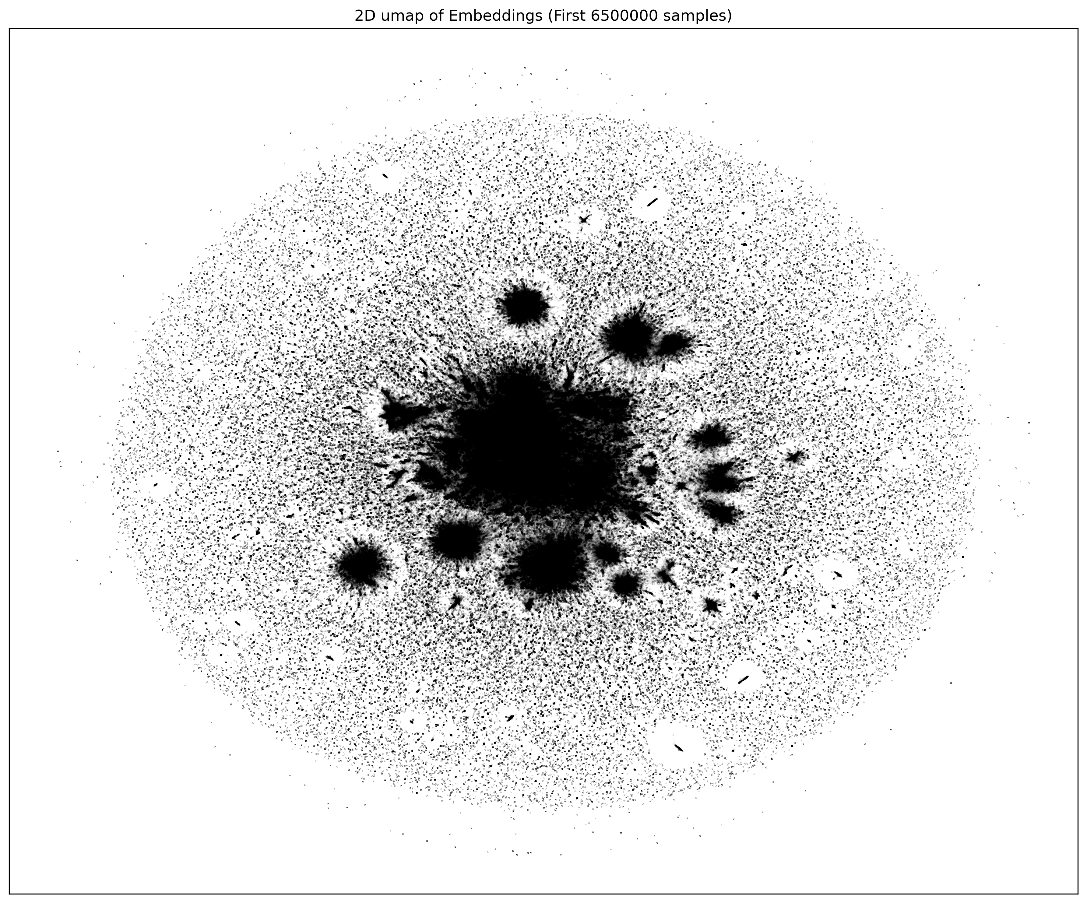
Finally, for UMAP, I had to rent out a bigger machine and thanks to the kind sponsorship of some credit from my internship. I rented out a Standard_E48s_v3 from Azure, this machine has 48 cores, 384 GB RAM and 768 GB disk. I ran only 6.5 million points through UMAP because 6.5 million was the closest I could get the machine before it went out of memory. I have a screenshot that shows all of the might of UMAP draining the RAM.

So finally, for the UMAP visualization, it looks like the following:

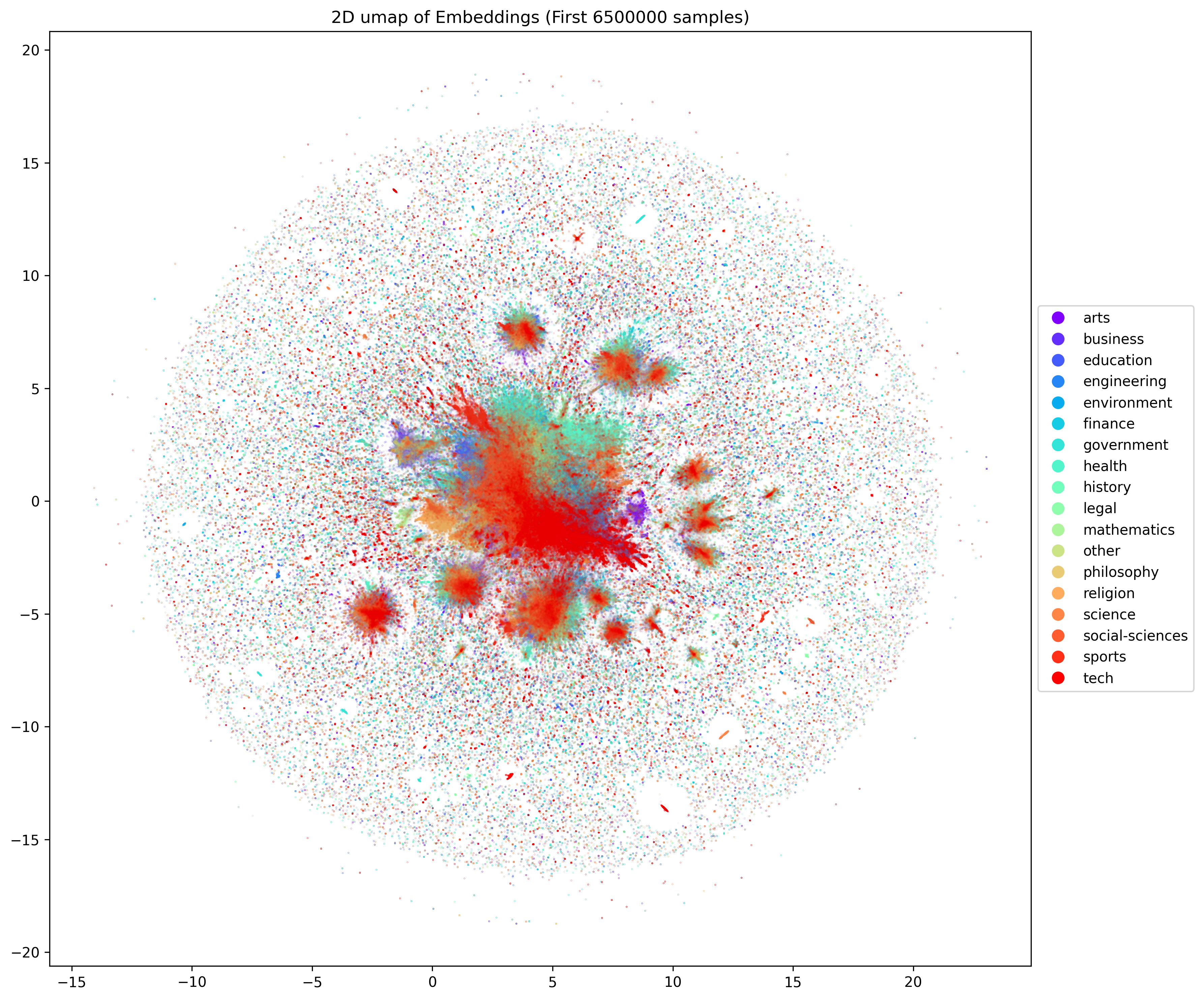
And the classifications look like this:

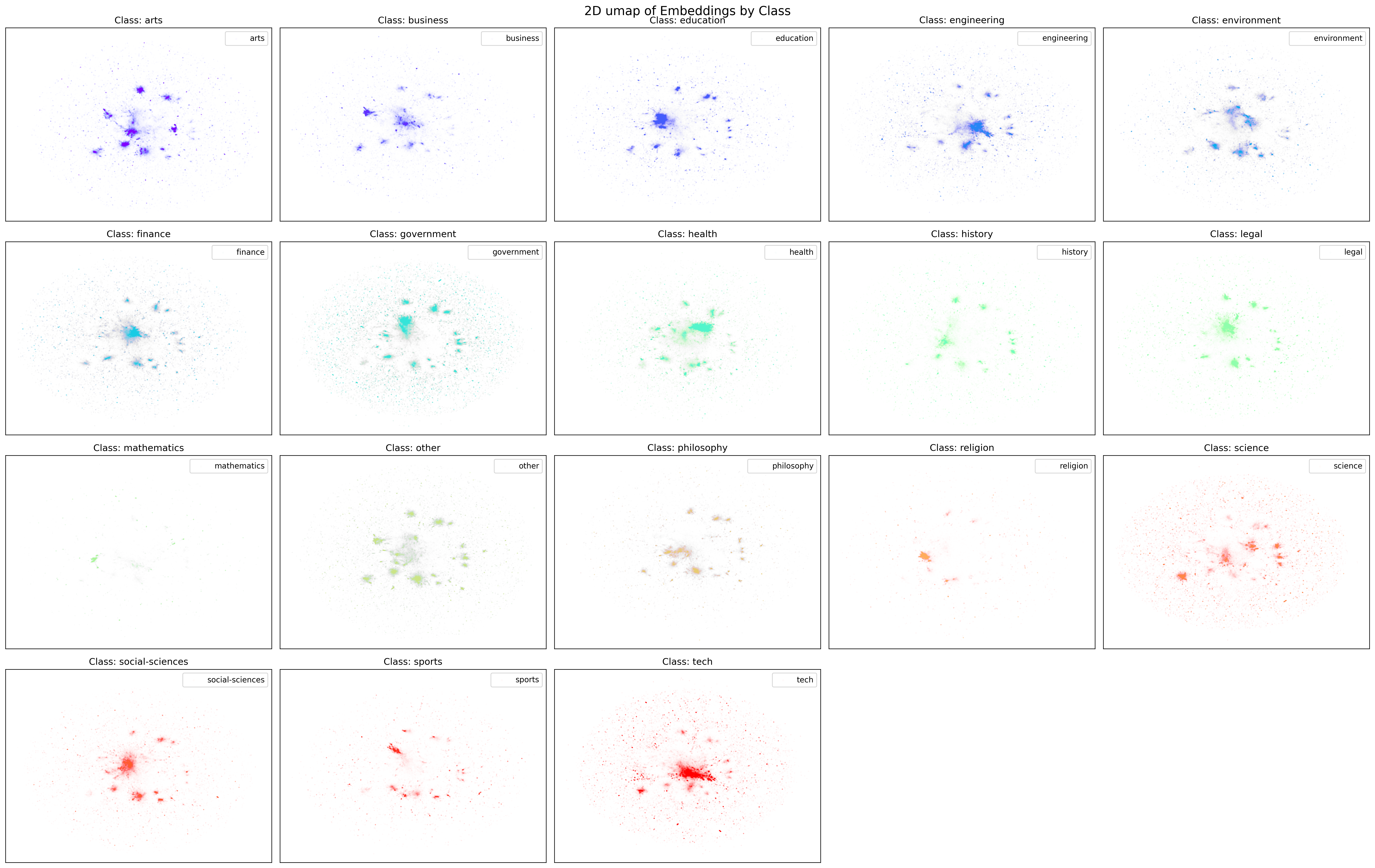
Per class plot looks like the following:

Conclusion

I feel like it was a fun experience to do overall but I could have done a little bit better. Specifically with the Deep Learning stuff. At the time I hadn’t rented a lot GPUs and I was just using my laptop, so I got desperate and decided to call it quits in the sake of time. This article is already pretty long as it is.

At the same time, its impressive to have gone this far. I really think that it is a big project that I got out this time. Considering that pdfs are a mixture of data and images, I think we are going to start seeing them more and more in training pipelines for VLMS/Omni models. If you want to try another massive dataset, you should try MINT-1T which has a mixture of PDFs + websites!

After all of this, I can confidently tell you that even now, I am pretty sure you can do a lot better and you can easily surpass this.

That is why, I am releasing all of the datasets in this huggingface repo. If you are just interested in the embeddings, you can find them in Kaggle right here. If you want to take a stab at the original dataset, the data card with download instructions can be found at this s3 bucket. Finally, if you want to check my code, it is currently in my monorepo right here.

Footnotes

Back to articles