Differential Evolution + CLIP = Image Generation

I recently stumbuled again to the exceptional paper about Modern Evolution Strategies for Creativity: Fitting Concrete Images and Abstract Concepts. So I decided to add a bit of a twist to the original paper. Aside from using CLIP to generate the images, I changed the original pipeline from using Evolutionary Strategies (ES) to Differential Evolution (DE).

What is a CLIP?

You can think of CLIP as one of the best inventions of Modern Deep Learning. Why? Because it made it possible to search any image by their semantic meaning. What I mean here is that you can now search on your Photos Album the word “dog” and you will get back all of the images of dogs in your catalogue.

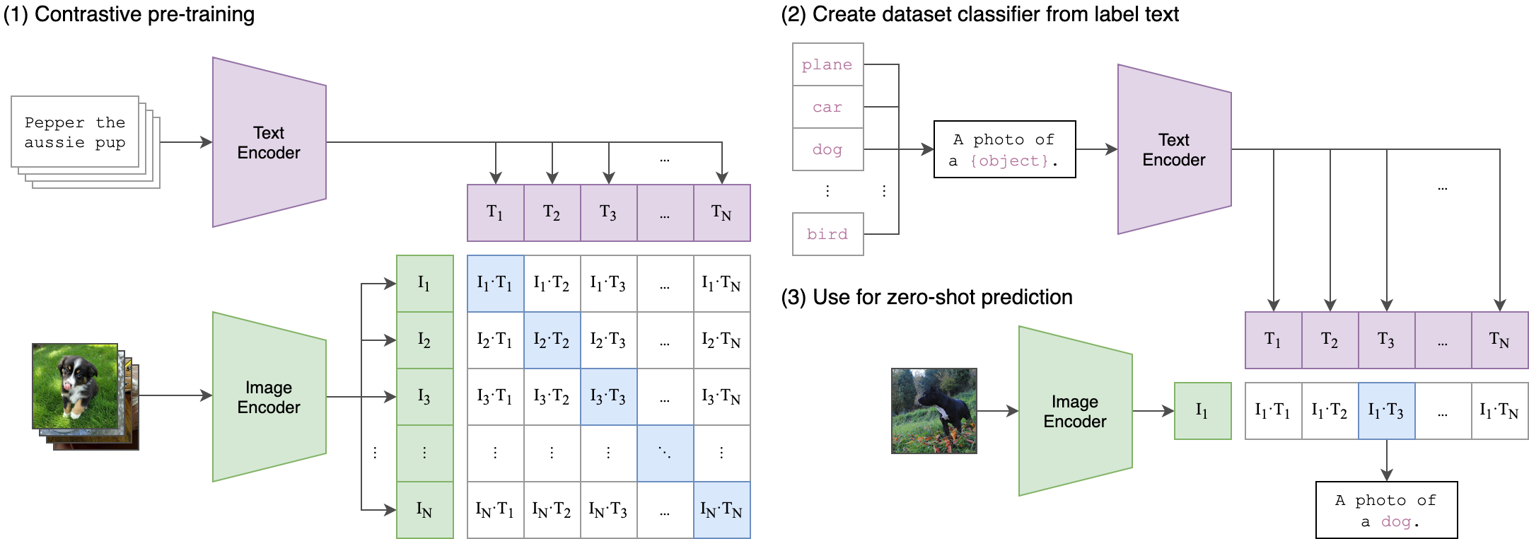
The way that this model works is by joining two encoders, one for the text and the other one for the image. The model is trained to predict both the image and the text as a pair.

The cool part about this models is that you can generate image and text embeddings separately when you are doing things like zero-shot prediction.

So, in this case, we are optimizing an image to resemble the embeddings of the text from the CLIP model during evaluation. This is great, because we actually don’t need to train the CLIP model, we just use it as an evaluator.

Differential Evolution

Differential Evolution (DE) is an evolutionary algorithm. All of the evolutionary algorithms work in a similar maner, they have four different stages: initialization, mutation, crossover, selection.

Initialization

The individuals are represented as a vector and they are in the search space that you particularly want. In this case we want to put down an RGB circle. So our vector would be constrained by the following: from 0 to 255 for the colors, from 0 to 10 for the size of the radius and from 0 to 255 for the coordinates x and y.

The formula to initiale all of the individuals and each of it’s parameters is the following:

x_kⁱ = x_k^min + r(x_k^max−x_k^min)

Where r is a random number between 0 and 1 and x_k^max and x_k^min are respectively maximum and minimum values for each parameter.

Mutation

The mutation is pretty simple, you grab three different members of the population x^r1, x^r2, x^r3 and generate a new individual vⁱ:

vⁱ = x^r1 + F(x^r2−x^r3)

Where F is a random number between 0 and 2.

Crossover

You combine the original vector xⁱ with the new generated vector from the mutation vⁱ and create another new vector called uⁱ.

You generate a probability of Crossover Cr and for each parameter you generate a random probability between 0 and 1 where if it is less than the parameter you select the new value v_k otherwise you select x_k

Selection

You select the best individual between uⁱ and xⁱ.

Putting it all together

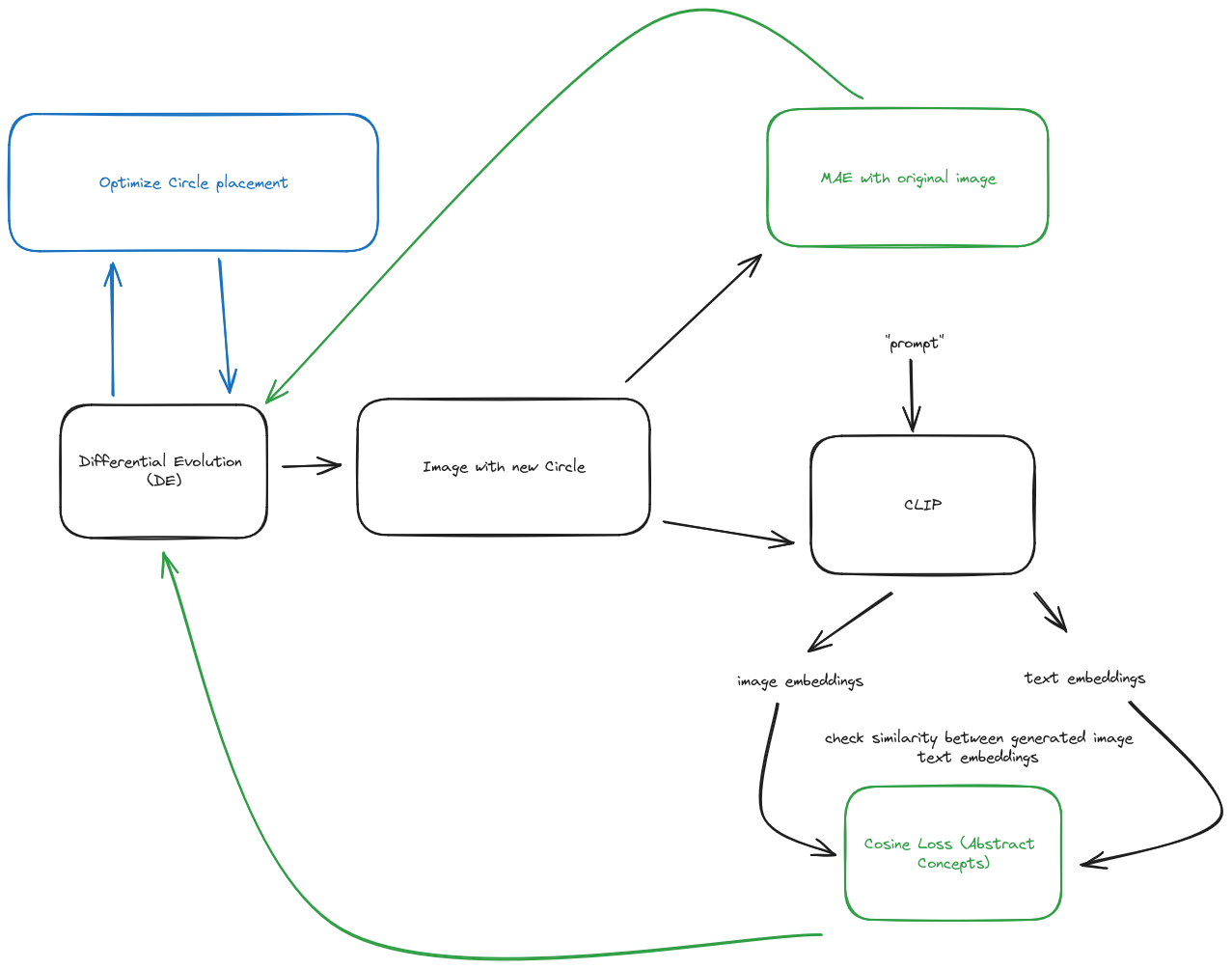
The pipeline looks similar to the original paper, but I decided to go with an approach similar to pointillism instead of cubism as they did in the original paper.

The way that this works is by optimizing the placement of a single point in the canvas and then placing it. Do that for 1000 points and you can get some abstract images! I have two different pipelines, one to approximate images and the second one is for approximating abstract concepts.

For approximating images, I used Mean Abstract Error (MAE) to approximate the pixel difference between one image and the canvas being generated.

For abstract concepts, I used cosine loss to view the similarity between the two vectors generated by CLIP, one for the text and the other one for the generated canvas. The closer they are, the more the image is supposed to look like the original concept.

The following is the loss function that I used for the cosine loss:

        def cosine_loss(genome, background, text, processor=processor, model=model):
          background = background.copy()
          genome = np.abs(genome.astype(int))
          x, y, r, R, G, B = genome
          r = max(4, r)
          color = (int(R%256),int(G%256),int(B%256))
          res = cv2.circle(background,(x,y), r, color, -1)
          with torch.no_grad():
            image_inputs = processor(images=res, return_tensors='pt')
            text_inputs = processor(text=text, return_tensors='pt')
            image_inputs, text_inputs = image_inputs.to('cuda'), text_inputs.to('cuda')
            image_features = model.get_image_features(**image_inputs)
            text_features = model.get_text_features(**text_inputs)
        
          cosine_similarity = torch.cosine_similarity(image_features, text_features)
          cosine_loss = 1 - cosine_similarity

        return cosine_loss.item()
      

Experiments

For the MAE pipeline it gets the job done and it looks great! Fitting something like the Monalisa over 10k steps looks great.

For abstract concepts, the pipeline actually doesn’t work as I was expecting. Here are some of the results with respective prompts:

The model actually never stopped optimizing.

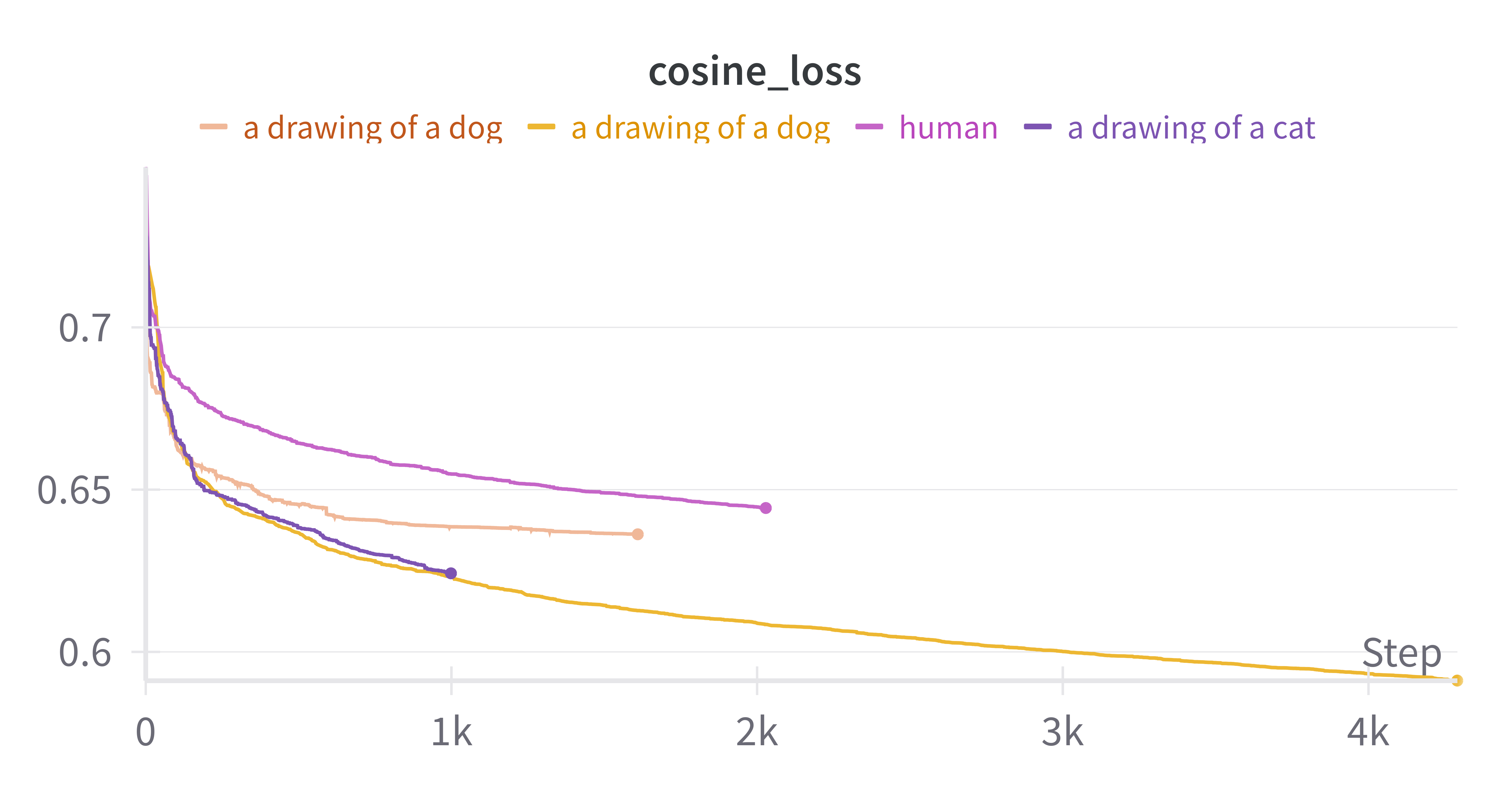
Here are the loss curves for each of the different functions and as you can see, they look super smooth.

Even if you don’t like it, this is what peak dog looks like after 4k steps using DE.

Conclusion

Although the results are certainly more abstract than what I was expecting, I think I found a way to do an adversarial attack against CLIP models. Just keep running the code for a couple of more days and you would find a horror that CLIP thought is a dog.

I recently started using connected papers so I want to be on this rabbithole a bit more. I want to replicate CLIPDraw by my own before moving on to other subjects.

If you would like to take a closer look into the code I created, it is own my Monorepo named m. And if you would like to check out a tiny blogpost about a gif generator I created for this blog post, that blog post is on my weblog, because is a super quick entry.

Back to articles